Our overbuild factor relative to maximum seasonal demand, not relative to average demand, is 1.52. That's the ratio of our maximum annual energy production capability (“peak capacity”) to our nationwide maximum demand during August when air-conditioners are working hard. August’s seasonal maximum power demand is about 768 GW.61  So the factor now is 1167 GW ÷ 768 GW = 1.52.

The 100% WWS Plan can perhaps help with the seasonal maximum demand problem by the practice of demand management, usually called demand response - DR.  For example, by shifting some daytime air-conditioning demand into the night, using chilled water and futuristic phase-change material technologies. DR can't shift between seasons of course, but it can shift between hours, thereby making August’s day-time demand not so peaky.

The author has no mathematical modeling tool at his disposal, so must be reduced to a seat-of-the-pants estimate of the necessary overbuild factor for an all-electric society energized mostly by unreliable sources.

It seems to me the intermittency issue by itself would require our present 2.5 X overbuild factor to be boosted to some value between 3 X and 4 X.  Changing from 1080 GW of always-on power to only 68 GW of always-on power gives me shudders. (In Table 2, rows 4 and 5, geo + hydro = 4.26% of 1591 GW =

67.8 GW).  But I'll swallow hard and place my bet on 3 X overbuild, as sufficient to cope with drastic reduction of always-on electric sources.

Then comes the matter of 100% of primary energy going to feeding the electric grid, not merely 39% as today.  This proportional expansion by a factor of about 2.5 probably doesn't require another factor-of-2.5 increase in the already-greater overbuild from the previous paragraph. (Remember though, that it does require a substantial increase in absolute production capability, “peak capacity”, from 1167 GW in 2015 to 1591 GW in 2050, per the Plan.)

As described above, DR can accomplish intra-day hourly shifting among sectors' demands.  For example, it can guarantee charging EV batteries only at night, and accessing commercial refrigeration facilities mostly at night (maybe lots of midnight-shift job openings in the food-distribution industry). It can shift into night-time the process of water-chilling for use as the next day's air-conditioning; and other demand-response management activities via the internet of things. 

So one might guess that the additional factor of increase in overbuild can be just 1.2 X or 1.5 X.  That is to say, the 3 X overbuild factor contingent on intermittency of fuel sources, stated in an earlier paragraph, must itself be boosted by another factor of 1.2 X or 1.5 X.  Thereby giving us an overall overbuild factor of 3.6 X to 4.5 X.

Let that be my offer.  For talking /disputation purposes, I will call it 4 X.

Hear ye, all environmentalists of weak faith in computer modeling 35 years into the future anticipating unproved technologies.  Join with me in arguing that 1591 GW of production capability is grossly insufficient.  Instead we would need 4 X 1591 GW = 6364 GW of production capability, in order to run the whole USA on a fossil-free and nuclear-free regime.

Ouch!  That overall $15.2 trillion construction cost that we were bandying about? It's really 4 X $15.2 T = about 60 trillion dollars.

That 67,500 km2 for utility-scale PV solar? It's really 4 X 67,500 km2 =

262,800 km2 (101,500 sq mi). In other words, almost all of Arizona.

Onshore wind? Better not to ask.  (Hint: Thank our stars for Thomas Jefferson. His 1803 Louisiana Purchase makes a nice dent in the reckoning.)

Another Course of Action - Nuclear

Of course we can't consider committing such wreckage upon our ecosystems and landscapes. It would be an ecocidal maniac who would really begin working toward a goal of 6364 GW, under the justification of "preserving the American way of life", or such nonsense. It would be hardly worth living at all, let alone "the American way”, if the only way were to defile our lovely land with 6364 gigawatts worth of windmills and solar panels.

But do acknowledge that the 100% WWS Plan points the way to reducing our society’s PRI-NRG consumption to just 1591 GW-y /year, down from 2010’s 3261 GW-y.51  Let us be appreciative to the Plan’s authors for urging us to aspire to that 1591-GW goal through 100% electrification of all energy sectors with elimination of all fossil fuels.  On that score they deserve "A" for effort.

Our objection to the Plan isn't their societal /ecological goal.  It's the klutzy method they have chosen to pursue that goal. Namely the land-hogging, material-intensive, GHG-emitting, expensive, diffuse-energy, low-density sources they’re using for their solution.  Why such klutziness, when we have available to us a compact-size, low-material, low-CO2, concentrated energy, high-density energy source like nuclear fission?

Nuclear Generation 3+ technology, under construction right now and typified by the Westinghouse /Toshiba model AP1000 pressurized water reactor, can achieve the Plan’s 1591 GWavg of national PRI NRG a lot more elegantly.  Meaning a lot less material, a lot less occupied land, and a lot less money.   

And because it's always-on nature is even more definite than fossil combustion, Generation 3+ nuclear won't require 3 or 4 X overbuild factor. We can probably maintain the 2.5 X overbuild factor that works satisfactorily for us now with our old-fashioned fossil technologies.

Moreover, if we do eventually change our electricity structure to a more distributed model, with smaller generation plants more widely distributed, we can then almost certainly reduce our overbuild factor to less than 2.5 X.

Generation 3+ small modular reactors - SMRs - are just around the corner. They will have the same passive-cooling and safety features as the 1100-mega- watt model AP1000.  SMR development is tending toward 250-megawatt capacity,62 so their land footprints will be only a fraction of the AP1000's footprint, which is itself less than 200 by 200 meters - 10 football fields.

SMRs’ very small footprint will allow them to be dispersed to individual neighborhoods, adjacent to the loads that they serve. Such a distributed-power electricity system is expected to be naturally more stable and reliable than the 20th-century concentrated-power electric grid model that drove the overbuild factor as high as 2.5 X to begin with.

But before we look forward to those happy days, let us examine the presently available AP1000 reactor, with regard to its land-use, material consumption, and money cost.

The Model AP1000 Pressurized Water Reactor:

Land, Material and Money

Land and material for an AP1000 are cut-and-dried. One reactor site (not counting the surrounding security zone) occupies less than 0.04 km2 (200 X 200 meters); the structure uses 15,500 tonnes of steel and 248,000 tonnes of concrete for its construction.63

AP1000’s cost is an article of contention. The Vogtle Georgia site where two such reactors are to be built is priced at $14 billion, giving a $7 billion

per-reactor cost.

But the Sanmen China site 150 miles from Shanghai has two model AP1000 units nearing completion, one in 2016 and the second in 2017. China National Nuclear Corporation - CNNC - will not commit to an estimate of Sanmen’s completed cost.  But CNNC’s own proprietary design of Generation 3+ pressurized water reactor, a smaller 650-MW unit, has been finished and is generating power now.  It’s located on Hainan Island, 300 miles from Hong Kong in the Tonkin Gulf, alongside another identical unit scheduled on-line in 2017. 

With combined capacity of 1300 MW, the pair have expected completed cost of $3.15 billion.64  Normalized to an 1120-MW AP1000, that’s equivalent to one large reactor costing $2.7 billion. [1120 MW ÷ 1300 MW X $3.15 B = $2.7 B]

The 100% WWS Plan’s Table S14 on page 91 cites several cost studies that range from $5583 /kW to $6640 /kW in the near-term for advanced pressurized water reactors - APWR - like the AP1000. Future-cost studies on page 92 project $3800 to $6511 /kW.

The cost figures have a wide spread, as usual. For discussion we will set aside the low China figure, though their low price is corroborated by South Korea’s experience at about $1700 /kW (accepting the official currency exchange) for a similar Gen 3 reactor,65 suggesting just $1.9 billion for an AP1000-size unit.

But current evidence of Korean nuclear technical /industrial expertise is the United Arab Emirates project now being built by Korea Electric Power Co - KEPCO.  That project involves four of the KEPCO-designed model APR-1400 reactors, for a reported price of $20.4–$25 billion. 65 .5 The first of its four reactors is nearly complete, scheduled to start up in 2017.

Normalized to the 1120-MW AP1000 reactor, KEPCO’s UAE bid cost (assuming midrange price of $22.7 billion) is $4.5 billion per reactor. 

[4 X 1400 MWp = 5600 MWp; $22.7 B ÷ 5600 MWp = $4.05 /Wp;  $4.05 X 1120 MWp = $4.5 B per AP1000 reactor]

In the interest of non-impeachability, we will simply average all eight of the American near-term and future costs published by the Plan, giving $5532 /kW as our working figure.66  Going forward to 2050 then, expect AP1000s to average $6.2 billion.   [1120 MW X $5532 /kW = $6.2 B]

The Gen 3+ design requires less frequent fuel changes than older-design reactors, enabling the AP1000 to perform at 93% CF.67 Its average power will be 1120 MWp X 0.93 = 1040 MWavg.

The 100% WWS Plan’s goal of 1591 GWavg PRI NRG could thus be achiev-ed by 1530 reactors acting alone.   [1591 GWavg ÷ 1040 MWavg = 1530] 

However, our already installed wind, hydro and solar capacity can supply a small portion of that demand.  In 2015 their contributions were:

Wind: 21.8 GW-y67.3(4.7% of 2015’s electric demand)

Hydro: 28.7 GW-y67.5(6.2% of 2015’s electric demand)

Solar: 4.6 GW-y67.7(1.0% of 2015’s electric demand)

Total WWS: 55.1GW-y   (11.9% of 2015’s electric demand)

With WWS making its small contribution the nuclear fleet would need to supply only 1591 – 55.1 = 1536 GWavg. 

There is one final consideration regarding the Plan  It proposes to use 11.48% of its grid power, 182.6 GW, to produce elemental hydrogen by electrolyzing fresh water.67.8 The hydrogen is intended for two applications:

1) Combustion with oxygen to attain very high temperatures, above 1000 deg C, for certain industrial processes.  About 23% of hydrogen production is intended for this purpose, consuming 41.0 GW of grid power.

2) Fuel-cell electric vehicles for heavy transportation.  About 77% of hydrogen production is so intended, consuming 141.4 GW of grid power.67.9 Presumably the Plan’s authors assess the U.S. trucking industry as competent to safely manage hydrogen tanks on their fleets.  The general automobile-driving public does not qualify of course.

Process heat application 1) is justified.  Generation 3+ Advanced Passive reactors cannot achieve temperatures in that range.  So even though water electrolysis for hydrogen results in a large portion of the 41.0 GW grid demand being wasted as heat, that is unavoidable.

Figure C

Fuel-cell transport 2) is quite inefficient, with the water electrolyzer /fuel-cell combination in Figure C showing only 25.6% electric-to-electric conversion efficiency.  That is to say, of the 141.4 GW grid load, only 25.6%, or 36.2 GW actually reaches the drive motors that propel the trucks.  The other 74.4%, or 105.2 GW, is emitted as waste heat into the environment.  By replacing fuel cells with batteries for electric vehicle trucking the all-nuclear grid reduces its power demand by that 105 GW wasted amount.

Thus the nuclear demand of 1536 GW after WWS contribution can be further reduced to 1431 GWavg.  [1536 GW – 105 GW = 1431 GW] 

Therefore only 1376 reactors are required.  [1431 GWavg ÷ 1040 MWavg = 1376]

Money:

At $6.2 billion per reactor, multiplied by 1376 reactors, the nuclear path would cost $8.5 trillion. Gen 3+ Advanced Passive nuclear

Which is quite a better deal than the $15-or-so trillion figure that jumped out at us for a WWS build-out.

It must be acknowledged that building 1376 reactors in 35 years is a daunting task.  It would mean 39 reactors per year, which far exceeds France’s

3.7 reactors per year built between 1973 and 1988.  Their 15-year performance has been the world’s most productive nuclear build-out.  On the other hand, US GDP is about 7 X greater than France’s.

The recently published China five-year plan envisions building 7 new reactors each year from 2015 to 2030.68  So it may be that 39 reactors per year for America in unrealistic.  Well, 35 years is just an aspiration.  Even if it takes

70 years, the thing is to get started.

In order to make comparisons of material, CO2 and land, we now summarize for the nuclear choice:

Gen 3+ Nuclear Plan

Steel: 1376 reactors X 15,500 tonnes steel = 21.3 million tonnes steel

Concrete: 1376 X 248,000 tonnes concrete = 341 million tonnes concrete

CO2:   21.3 M t X 1.8 t + 341 M t X 1.2 t = 448 million tonnes CO2

Land: 1376 X 0.04 km2 = 55 km2 (21 sq mi, less than Manhattan island).*

Money: 1376 reactors X $6.2 B = $8.5 trillion Gen 3+ Advanced Passive nuclear

*For the foreseeable future, large reactors will be surrounded by security zones until technology evolves to permit underground placement of Small Modular Reactors - SMRs.  So the reserved site area for an AP1000 will be much larger than 0.04 km2.  For discussion purposes let us assume one-half square mile (1.3 km2) as fenced security zone area.   Then the amount of occupied land throughout the US would be 1376 X 1.3 km2 = 1790 km2 (690 sq mi).  That’s about half of Long Island, New York.

We will now compare these values to the 100% WWS Plan’s entire build-out, with use-values extracted from our previous sections.

Comparison of 100% WWS Plan to

Gen 3+ Nuclear Plan

Steel:

Utility PV:  186 M tonnes

Residential PV: 6.5 M t  (aluminum)

Commercial PV:    44 M t

CSP:        188 M t

Onshore wind:  188 M t

Offshore wind:  180 M t

Total Steel:  793 million tonnes 100% WWS Plan, entire

Concrete:

Utility PV:      negligible

Residential PV: none

Commercial PV: none

Onshore wind:  701 M t

Offshore wind:  673 M t

CSP:       605 M t

Total Concrete: 1979 million tonnes 100% WWS Plan, entire

CO2:

Utility PV:     11,400 M t CO2eq

Residential PV:  2300 M t CO2eq

Commercial PV:  1700 M t CO2eq

Onshore wind:    885 M t 

Offshore wind:  1133 M t 

CSP:        1060 M t

Total CO2eq:  18,500 million tonnes 100% WWS Plan, entire     

About 2.7 years of our BAU emissions.36

         

Land:

Utility PV:  67,500 km2   {perhaps less, per NREL’s packing factor approach in future}

Residential PV:  none

Commercial PV:  none

Onshore wind: 289,200 km2

Offshore wind:  69,500 km2 (ocean)

CSP:       19,200 km2

Total Land:  375,900 km2  (145,100 sq mi)

                                    {perhaps less, per NREL’s packing factor approach in future}

             86,700 km2 is unusable for agriculture or any other purpose.

                            That’s 1.1% of the lower 48 states. 100% WWS Plan, entire

Ocean:        69,500 km2  (26,800 sq mi)100% WWS Plan, entire

Money:

Utility PV:  $5.3 T

Residential PV:  $1.5 T

Commercial PV:   $0.9 T

Onshore wind: $2.6 T

Offshore wind:  $2.7 T

CSP:         $2.2 T

Total Money:   $15.2 trillion 100% WWS Plan, entire    

                             (Or $25.9 trillion per the Plan’s Table S14 sources.)

               Factor of difference             Percentage

                     WWS ÷ nuclear              nuclear ÷ WWS

Steel:                  793 ÷ 21.3  = 37.2 X                        21.3 ÷ 793 = 2.7%

Concrete:         1979 ÷ 341 = 5.8 X                        341 ÷ 1979 = 17.2%

CO2eq:           18,500 ÷ 448 = 41.3 X                448 ÷ 18,500 = 2.4%

Land:             375,900 ÷ 55 = 6830 X                 55 ÷ 375,900 = 0.015%

Money:           $15.2 T ÷ $8.5 T = 1.8 X                $8.5 T ÷ $15.2 T = 55.9%

Which begs the question: if nuclear beats WWS so dramatically on material usage (only 2.7% and 17.2%), why does it beat WWS less impressively on money cost? (55.9% of WWS cost)

Could it be that China and South Korea have it right? That when you get right down to building them, instead of paying financing charges and legal fees, they’re actually quite affordable, at $2.7 billion (China), or $4.5 billion (South Korea)?   If those Asians know something that we don't know, their nuclear advantage is 41% of WWS cost, in Korea. [$4.5 B ÷ $6.2 B X our 56% = 41%]

Only time will tell.

To visualize the advantages of the Gen 3+ nuclear course of action versus the 100% WWS Plan, Figure D presents bar graphs comparing material consumed, land occupied, and money expenditure.  Both American and Korean prices are shown.

Figure B.pdf

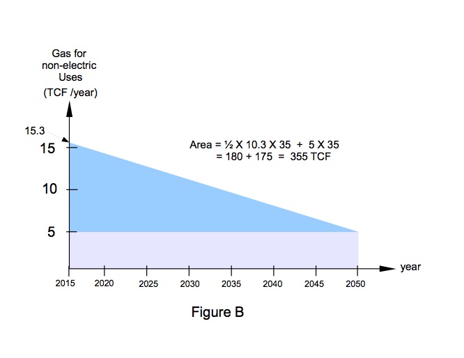
Estimated pattern of natural gas usage for purposes other than

electricity generation, during the 35-year Plan build-out. 

It can be graphically integrated to find non-electric

cumulative gas consumption through 2050.

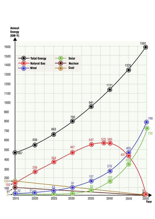
Figure D

Bar graphs of data from the tables above.

The solar and onshore wind land areas are from footnoted NREL published studies. 

The red and blue area bars do not represent land reductions that may be realized in future by NREL packing-factor approach to PV solar, or aggressive concentration of wind

in the great plains at the avoidance of hilly terrain elsewhere.

The yellow land area bar represents the entire secured site area,

not the reactor equipment proper.

The yellow money bars are calculated for a fleet of 1376 reactors rated 1120 MWp. 

Based on per-reactor price of $6.2 B (US) and $4.5 B (KEPCO).

Another Opinion on Dollar Cost

Besides CSP, the Plan’s Table S14 also provides an alternative source of cost figures to the NREL-sourced PV solar costs that we used earlier. And also alternatives to US DOE’s onshore wind costs, and to IRENA-sourced offshore wind.

Those numbers show rather a wide spread among scholarly studies, for every technology.  One can only average them to get a representative sense.  Doing so using both near-term and future (post 2014) figures for PV 48 provides the following other-opinion values, in units of $ /kWp: 49

Utility-scale fixed PV: $2077 /kWp-ac

Utility-scale tracking PV: $2683 /kWp-ac

Utility-scale PV average: $2380 /kWp-ac = $2.38 /Wp-ac

Residential rooftop PV: $3955 /kWp-dc = $3.96 /Wp-dc

Commercial rooftop PV: $3016 /kWp-dc = $3.02 /Wp-dc 

Using these working figures obtained from the 100% WWS Plan’s 2014 references, the other-opinion lifetime build-out costs become much greater than the PV solar costs obtained earlier from NREL’s model projections.  The costs are:

Utility-scale PV:  $2.38 /W X 2,326,000 MW = $5.5 trillion for initial installation.  Multiplying by our earlier-developed lifetime maintenance factor 1.8 gives

$9.9 trillion. utility PV - other opinion

Residential PV:  $3.96 /W-dc X 379,500 MW = $1.5 trillion initial.  Multiplying by lifetime maintenance factor 1.76 gives $2.6 trillion. residential PV - other opinion

Commercial PV:  $3.02 /W-dc X 276,500 MW = $0.8 trillion initial.  Multiplying by lifetime maintenance factor 1.92 gives $1.5 trillion. commercial PV - other opinion

Total PV solar:  $9.9 T +  $2.6 T +  $1.5 T = $14.0 trillion total PV solar - other opinion

This is completely at odds with the $7.7 trillion build-out cost obtained from NREL’s modeled price declines of PV solar.  We mention this other opinion for form’s sake.

Revisiting the Plan’s reference Table S14 for wind,50 but using only the lower future-build figures because we had already discounted by 20% our future estimated wind prices, gives other-opinion costs:

Onshore wind: $1822 /kWp  = $1.82 /Wp

Offshore wind: $3773 /kWp  = $3.77 /Wp

Here too the other-opinion lifetime costs are considerably higher than our DOE- and IRENA-derived figures stated earlier.

Onshore:  $1.82 /W X 1,701,000 MW = $ 3.1 trillion initial installation.  Adding our 20% lifetime maintenance expense gives $3.7 trillion.

Offshore:  $3.77 /W X 780,900 MW = $ 2.9 trillion initial.  Adding 30% lifetime maintenance gives $3.8 trillion.

Total wind:  $3.7 T + $3.8 T = $7.5 trillion total wind - other opinion

This in contrast to $5.3 trillion obtained from IRENA’s anticipated 20% reduction relative to wind-turbine construction costs in 2014.

Total W&S build-out cost using the other opinion:

By this alternative accounting, obtained from the 100% WWS Plan’s 2014 references for PV solar, onshore and offshore wind, and CSP solar, overall lifetime cost would be $21.5 trillion overall wind & solar - other opinion

  

Whichever figure we take, the Plan’s lifetime cost is in the range of

15 to 21 trillion dollars. Which is about equal to our Gross Domestic

Product - or greater than.

Keep always in mind, this is with zero overbuild planned into the system, so cannot be considered the final word.

For discussion of the potential for copper and silver to act as limiting factors in the WWS construction plan, jump forward to the end of this webpage.  Search for “Material Limits”.

The Wind and Solar Build-out Schedule: How Quickly?

The Plan's authors put forward an S-shaped building-schedule curve in Figure 5 on page 21. Its steepest slope, corresponding to the maximum construction rate, is for the period 2020 to 2025. The build rate slackens from 2025 to 2030, slows drastically from 2030 to 2040, then tapers to a crawl for the final 10 years.

Figure 5

Graph of the Plan’s proposed schedule for building wind and solar

generating capacity from 2015 – 2050, and for reducing demand.

The vertical axis variable can be regarded as annual average power,

such that US Primary Energy yearly consumption is that value,

in units of terawatt-years,TW-y.

The value 2.400 TW-y would more often be expressed as

2400 GW-y of energy, per year.

As presented, the graph misstates US Primary Energy

of the four societal sectors in year 2010 (objection).  

The correct value is 3261 GW-y.  (Footnote No. 51.)

Here is a deficiency.  The proposed nameplate capacities of wind and solar in those four rows combine to only 5035.2 GW (expressed as 5,035,200 MW). That amount of generating capacity would not be sufficient to produce 1401 GW-y annually, when operating at the present US Capacity Factors - CF - for utility-scale wind and solar production devices.(objection)  US wind & solar capacity factors were 29.7% for wind and 21.9% for utility solar in 2015.12  

At those capacity factors the total annual energy produced by the Plan's standard-demand utility-scale wind and solar facilities (rows 1, 2, 9, and 10) would be:

For wind in rows 1 and 2:  737.1 GW-y per year.  (0.297 CF X 2,481,900 MW combined capacity of rows 1 and 2)

For solar in rows 9 and 10:  559.2 GW-y per year.  (0.219 CF X 2,553,300 MW combined capacity of rows 9 and 10)

Utility-scale wind and solar combined will produce 737.1 + 559.2 = about 1296 GW-y. Thus there is a production shortfall from the 1401 GW-y expected in the “Percent of 2050 all-purpose load” column.(objection)  (1401 – 1296 = 105 GW-y shortfall)

Rooftop solar sources appear in rows 7 and 8.  Residential rooftop is expected to produce 3.98% of the total standard load (column 2), which would be 0.0398 X 1591 = 63.3 GW-y.

Residential PV solar capacity at the end of 2015 was 5.53 GWac.12.3  Its potential production was 5.53 GW  X 8760 h /yr = 48,440 GW-h.  Residential solar’s actual energy production in 2015 was 6999 GW-h.12.4  Thus US residential rooftop solar operated at capacity factor = 14.4%. (6999 GW-h actual ÷ 48,440 GW-h potential = 0.144)

Residential solar CF is low because of south-siting issues, angle of tilt, and partial shading by trees and other buildings.

On row 7 of Table 2, the Plan’s eventual residential buildout to 379,500 MWdc  will produce 322,600 MWac, operating at dc-to-ac conversion efficiency of 85%.  [379,500 MWdc X 0.85 = 322,600 MWac]  Look ahead to p. 10, Land Use Utility PV Solar , for discussion of the conversion efficiency of dc-to-ac inverters.

Therefore row 7’s residential equipment can be expected to produce yearly energy of 14.4% CF X 322,600 MW = 45.5 GW-y.  Not 63.3 GW-y as that row’s column 2 percentage anticipates, for a residential PV shortfall of 17.8 GW-y.(objection)  (63.3 – 45.5 = 17.8 GW-y)

Attending to commercial /government rooftop solar in Table 2’s row 8, the Plan expects to produce 3.24% X 1591 GW = 51.5 GW-y annually. 

Commercial /governmental /industrial distributed PV solar capacity at the end of 2015 was 6.00 GWac.12.5  Its potential production was 6.00 GW  X 8760 h /yr = 52,560 GW-h.  Commercial distributed solar’s actual energy production in 2015 was 7140 GW-h.12.6  Thus US commercial rooftop solar operated at capacity factor = 13.6%. (7140 GW-h actual ÷ 52,560 GW-h potential = 0.136)

The Plan’s row 8 commercial buildout to 276,500 MWdc multiplied by 85% conversion efficiency will provide ac capacity = 235,000 MWac.  At 2015’s capacity factor the equipment would therefore produce yearly energy of

13.6% CF X 235,000 MW = 32.0 GW-y.  Not 51.5 GW-y as that row’s column 2 percentage anticipates, for a commercial PV shortfall of 19.5 GW-y.(objection) 

(51.5 – 32.0 = 19.5 GW-y)

Summarizing, the combined wind & solar standard energy production of the Plan (rows 1, 2, 7, 8, 9, and 10), operating at 2015 capacity factors, would be 1296 + 45.5 + 32.0 = 1374 GW-y.  Not 1516 GW-y, which the Plan expects.   [1516 = 1401(rows 1, 2, 9 and 10) + 63.3(row 7) + 51.5(row 8)]

The few percent additional energy from hydroelectric and geothermal facilities (rows 3, 4, 5 and 6), amounts to only about 76 GW-y per year, taken from the percentages stated in that column.  That is to say, 4.77% of 1591 GW-y is about 76 GW-y.  Thus hydro and geo would boost the overall national total to only 1450 GW-y per year.  [1374 + 76 = 1450 GW-y /year]

As presented, the Plan therefore has insufficient wind and solar infrastructure to achieve its standard-demand production target of 1591 GW-y /year, when operating at the US capacity factors prevailing in 2015.(objection)

It may be that the Plan's authors are hoping for equipment-driven or weather-driven capacity factor improvements in the coming decades.  That may be a reasonable hope for turbine-blade technology advancement and by benefitting from very windy offshore placement of turbines.  But onshore weather conditions are likely to be countervailing due to lower wind speeds as earth’s atmosphere warms.

It would also be reasonable to expect US utility-scale solar capacity factor to be enhanced by aggressively concentrating new farms in our southern states, especially our southwest deserts and Florida.  But that doesn’t seem to be the Plan’s intent, referring to The Solutions Project Infographics for the 50 states.12.8 Those infographics seem to indicate that the states’ equipment mix dedicates an amount between 32% and 42% of the nation’s standard-demand solar facilities to the northern belt consisting of New York, New Jersey, Pennsylvania, Ohio, Indiana, Illinois, Michigan, and Wisconsin.12.9

Even by counting reserve peaking CSP from row 11, its additional energy capability does not nearly make up for Table 2's standard equipment deficiency.  With nameplate capacity of 136.4 GWp (“Name-plate capacity” column 3 heading), and assuming a very generous solar insolation capacity factor of 27%*, the Plan’s annual peaking energy production from CSP would be only 0.27 X 136.4 GW-y = 37 GW-y /year.

*Contingent on CSP placement in very sunny regions only.

Combined with 1374 GW-y stated above from standard-demand sources in rows 1 through 10, that peaking addition gives 37 GW-y + 1374 GW-y =

1411 GW-y /year.  So total US electric energy production (standard plus peaking backup) would still be about 180 GW-y less than the 1591 GW-y consumption value anticipated in 2050.  In other words, not only does the Plan provide zero standard overbuild, it yields a significant energy shortfall even with its backup /storage factored in.

This is not credible. The Plan's electricity infrastructure's energy content is proposed to be substantially greater than for our electric grid of 2015.  Namely 1591 GW-y, up from 1167 Gw-y in 2015, and it anticipates getting 97% of that substantially greater amount from unreliable sources.  Yet it reduces our 2.5 X overbuild factor in 2015 down to no overbuild at all.  As presently structured, it cannot succeed.

Later, this study will suggest a reasonable overbuild factor, after first performing a detailed analysis of the Plan’s material usage and costs. That overbuild suggestion will be considerably larger than 2.3 X.  It seems indisputable to the author that such an increase in overbuild will be necessary to compensate for changing the character of our energy sources from always-on performance to intermittent performance.

Setting aside the overbuild issue for the time being, let us consider a possible build-out schedule for only that inadequate equipment which is proposed in Table 2. Given the 35-year duration, it is not possible to attack the build-out challenge in a linear fashion, by building 1 /35  of that equipment in the very first year, say 2016. There is not sufficient wind-turbine manufacturing capacity in the entire world to build 1 /35 of 484,200 turbines in a single year (rows 1 and 2 of Table 2, column headed “number of new plants or devices”). That would call for 484,200 ÷ 35 = 13,800 turbines, each one a 5-MW behemoth, to be built in a single year.

Our best-ever year for wind construction was 2012, when we added 13.1 GWp.13  At 5 MW per turbine, as called for in the Plan, year 2012 achieved the equivalent of 2620 such giant turbines.  [13.1e9 Wp ÷ 5e6 Wp = 2620 turbines]   Thus the 13,800 turbines that would be needed to jump off to a linear beginning would be 5.3 X greater than our all-time best year. That's impossible.   

[13,800 turbines ÷ 2620 turbines = 5.3]

Even more so for solar panels. 2015 was our best year ever, with 6200 MWp-ac of new capacity installed.14 But 1 /35 of 2,982,000 MWp (rows 7, 8 and 9 combined from Table 2) would require 85,200 MWp to be constructed in the first year.  [2,982,000 ÷ 35 = 85,200 MWp]  Such a factor-of-13 jump would be even more impossible than the factor of 5.3 for wind.   [85,200 MWp ÷ 6200 MWp = 13.7]

To tackle the Plan’s building project we would need to begin with the manufacturing capacity that we now possess, then continually construct more manufacturing plants year after year.

If the inertia afflicting American society could be overcome, the jealous withholding of material and financial resources and the paralysis of political will, it would in principle be possible to increase turbine and solar panel production exponentially.  The phrase “increase exponentially” means to achieve an annual growth rate, some percentage, that compounds year-by-year.

Let us carefully consider that task for the wind buildout proposed in Table 2. 

a) Onshore wind plus offshore wind is intended to produce 50.0% (add rows 1 and 2) of US average load for year 2050, which is 1591 gigawatt-years per year (bottom row of Table 1, referenced above).  Thus 0.50 X 1591 = 796 GW-y, generated in the year 2050.

b) In 2015 actual US wind energy production was 21.8 GW-y.15  This is the initial value from which we would start compounding.

c) To grow at a compounded rate that boosts 21.8 to 796 GW-y /year would require an annual growth rate of 10.826%.  Which implies a factor of increase equal to 1.10826, exponentially compounded.  21.8 X (1.10826)35 = 21.8 X 36.51 = 796 GW-y.

This exponential growth curve of wind energy is the blue line in the Figure A graph.

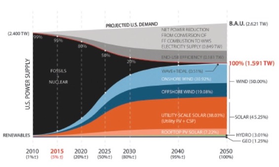
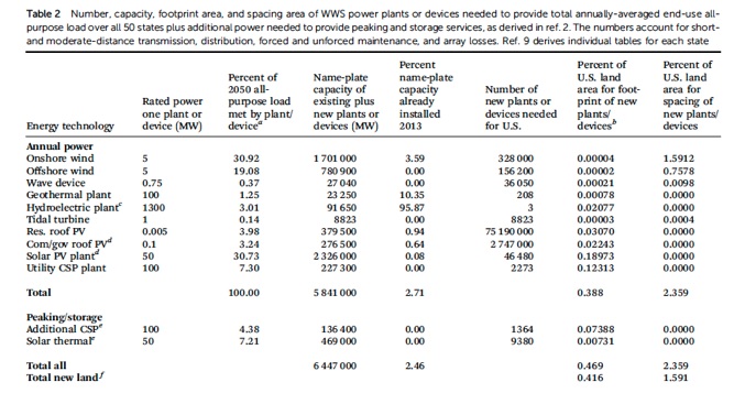
7.5 megawatt wind turbine

200-meter hub height

wind farm in UK

http://tinyurl.com/hzuh27g

Download PDF

Download PDF

Download PDF

Download PDF

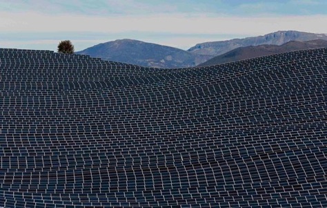
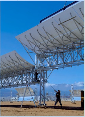
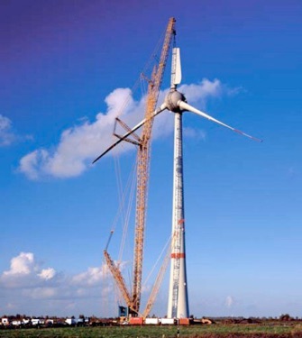
Table 2 of the 100% WWS Plan. 

Page 6 of the published study; frame No. 8 of its PDF document.

https://web.stanford.edu/group/efmh/jacobson/Articles/I/USStatesWWS.pdf

Download Table 2

parabolic-trough CSP

reflector-mirror

PV solar panels swarm

California hillside

Figure A

Various energy sources during the 100% WWS Plan’s 35-year build-out. 

The building schedules for wind and solar are here presumed to be exponential.

The natural gas-for-electricity red curve accounts for hydro’s contribution.

 

That red curve can be graphically integrated to find cumulative natural gas consumption through year 2050.

Download Figure A

Mr. Todd De Ryck has been kind to reconstruct this web page using WordPress.

In that form it may be more sharable.  It can be seen at

 https://thstlewpg.wordpress.com/2016/09/17/tim-maloneys-analysis-and-critique-of-100-wws-for-usa/

To achieve such a schedule, we would need to prodigiously expand our manufacturing capacity for PV panels and for wind turbines by year 2020.  Is that feasible?

To address this question, let us quantify the build-out rate represented in Figure 5 for the 2020–2025 period. Then we can compare that hoped-for build-rate to what has been accomplished so far, to 2015.

Before beginning this task, we must register an objection to Figure 5 regarding its vertical scale value 2.400 TW for US Power Supply ("end-use power demand for all purposes" in the figure caption). That 2.400 value would imply US annual PRI NRG of 2400 GW-y for year 2010.

But actual US PRI NRG for 2010 was 3261 GW-y, per the Energy Information Administration - EIA. They state 2010’s PRI NRG as 97.48 quadrillion BTU's,51 called Quads.  With conversion factor 1 Quad = 33.456 GW-y, we actually consumed 97.48 Q X 33.456 GW-y /Q = 3261 GW-y.

Thus the correct PRI NRG values pertaining to the US for years 2010–2050 would be greater than the values shown in Figure 5, by a factor of 1.36.  [3261 GW-y ÷ 2400 GW-y = 1.36]   We will deal with this error by obtaining graphical scaled values from Figure 5 as it is presented, then multiplying all such results X 1.36 to represent our country’s reality.

There are six data points that must be extracted from Figure 5 to enable calculation of build-rates for solar and wind during the 2020–2025 period.  They are:

Data Point (1): The bottom point of the orange regions at year 2020. This point represents the tiny bit of PRI NRG supplied by hydro and geothermal in 2020, to which the orange solar regions add their contributions. That value cannot be scaled because it's so tiny, but we can estimate it as about 1.5% of US PRI NRG because we know from EIA that hydro plus geothermal contributed 0.9% in 201052 and in 2015.53 We will suppose that 2015’s contribution of 0.9% can grow to about 1.5% by year 2020 (though hydro has been decreasing lately).54

Thus, in Figure 5 we will call the value at the bottom of the orange region as 0.015 X 2400 GW-y = 36 GW-y.

Data Point (2): The top point of the orange solar regions at year 2020, which is also the bottom point of the blue wind regions. This value, with 36 GW-y subtracted from it, represents the PV and CSP solar contribution to US PRI NRG during the year 2020 (before adjustment X 1.36, as for all graphical data points that we extract).

This data point (2) also lays the basis for finding the contribution made by wind in the year 2020.

Data Point (3): The top point of the blue regions at year 2020.  This value, with the bottom point of the blue regions subtracted from it (Data Point No. (2) represents the wind contribution in year 2020.

Data Point (4): The bottom of the orange regions at year 2025.

Data Point (5): The top of the orange, bottom of the blue regions, at year 2025.

Data Point (6): The top of the blue regions at year 2025.

Performing mechanical ruler scaling at points 2 and 3, and at points 5 and 6, we obtain:

Point (2):   254 GW-y       extracted graphically

Point (3):   449 GW                    “

Point (5):   566 GW-y                 “

Point (6):  1034 GW-y                “

Data Point (4)’s value also is too tiny to be scaled. We will estimate it very optimistically as 2.0% of 2010’s PRI NRG, so 0.02 X 2400 GW-y = 48 GW-y.

Data Points (2), (3), (5) and (6) taken from Figure 5 must be corrected to actual US PRI NRG values by multiplying X 1.36.  We obtain

Point (2):  345 GW-y             corrected X 1.36

Point (3):   611 GW-y                       “

Point (5):   770 GW-y                       “

Point (6):  1406 GW-y                      “

Data Points (1) and (4), 36 GW-y and 48 GW-y, are valid as stated above because they were not obtained from erroneous graph-scaling.

We thus conclude the following quantities conveyed by the Plan's S-shaped building schedule.

For year 2020:

Solar contribution to PRI NRG would be 309 GW-y.   [345 – 36 = 309]    [corrected Point (2) minus Point (1)]

Wind contribution to PRI NRG would be 266 GW-y.   [611 – 345 = 266]    [corrected Point (3) minus corrected Point (2)]

For year 2025:

Solar contribution = 722 GW-y.   [770 – 48 = 722]   [corrected Point (5) minus Point (4)]  [represented by width of expanded orange regions]

Wind contribution = 636 GW-y.  [1406 – 770 = 636]  [corrected Point (6) minus corrected Point (5)]  [represented by width of expanded blue regions]

So by careful use of the Figure 5 graph, we find for the 5-year period 2020– 2025:

The building rate for solar would have to be [722 GW-y (in 2025) minus

309 GW-y (in 2020)] ÷ 5 yr  = 82.6 GW-y /year for solar, obtained graphically.

The building rate for wind would have to be [636 GW-y (in 2025) minus

266 GW-y (in 2020)] ÷ 5 yr  = 74.0 GW-y /year for wind, obtained graphically.

Throughout the above derivation we have accepted the relative widths of orange to blue as properly drawn in the early part of the build-out (years 2020 – 2025). We have done so despite their being improperly drawn(objection) for year 2050. Orange is drawn wider than blue at 2050, though producing less energy. That is, orange PV and CSP solar produces only 45%, versus blue wind's production of 50%. (Refer to “Percent of 2050 all-purpose load met by plant /device” in Table 2.) Therefore blue should be drawn wider than orange.

The building rates extracted above from Figure 5's S-curve have been interpreted in Energy units (GW-y).  That is equivalent, in purport, to interpreting in Average Power units (gigawatts average, symbolized GWavg, strictly speaking).

However, renewables build-out rates are almost always denoted in peak units, symbolized GWp, strictly speaking.  Usually verbalized as "peak capacity" or just "capacity".

To render a nation's energy units (equivalent, in purport, to a nation’s average power) into the nation's peak capacity units, we must know the nation's average capacity factor CF for that particular technology.

For the US in year 2015, per EIA and Solar Energy Industry Association - SEIA - average capacity factors were:

PV (all 3 placements) and CSP solar: 18.3%55

Wind: 29.7%56

Total solar CF was mediocre because low-CF residential and commercial distributed solar are still a substantial portion of the US capacity in 2015. Utility-scale systems, with their proper south-facing panel orientation, would far surpass residential and commercial capacity in the Plan's implementation. Well situated PV and CSP utility farms can achieve insolation capacity factor percentages in the low-twenties (mid-twenties in southwest US).   

We will assume 23% CF as the expected nationwide average for our aggregate solar equipment after year 2020. That value is appropriate for large-project PV solar's ac peak capacity, and for large-project CSP’s entire solar-field insolation energy (eschewing the artificially reduced /restricted solar-field energy that is usually published).

New wind installations perform better than the average of the entire US wind fleet, which naturally contains many older, smaller machines. The American Wind Energy Association - AWEA - and the US DOE have put forward a

32% – 35% range of capacity factors expected for new wind farms.57 For discussion purposes we will assign the value 33.5% from the middle of that range.

With those two capacity factor assumptions, 0.23 solar and 0.335 wind, expected for the 2020–2025 building period, and referring to the graphically obtained solar and wind building rates expressed in energy units above, the required annual rates of peak capacity construction become:

Solar:  82.6 GW-y /year ÷ 0.23 = 359 GWp-ac /year

Wind:  74.0 GW-y /year ÷ 0.335 = 221 GWp-ac /year

2016 was our best-ever year for PV solar installation with 14.63 GWp-dc added,14 implying about 12.43 GWp-ac with conversion efficiency of 85%.  Therefore the 100% WWS Plan intends to ramp up our solar panel manufacturing capacity (or China's) from 12.43 GW to 359 GW, a factor of 29X, within the next 5 to 10 years.  This is not credible. (objection)

For wind, 2012 was our best year ever, with 13.1 GWp added.13 This means that the Plan's authors intend to simultaneously ramp up somebody's wind turbine manufacturing capacity from 13.1 GW to 221 GW, a factor of 16.9, also within 5 to 10 years. Not as preposterous as solar, but still not credible. (objection)

Perhaps the 100% WWS Plan’s wind ambition can be best appreciated by specifying individual wind towers /turbines. Taking the Plan's 5-MW per machine, 2012 saw the equivalent of 2620 such turbines built in the US.  [13.1 GW ÷ 5 MW = 2620]  By 2020 – 2025 that installation rate would need to increase to 16.9 X 2620 = 44,300 turbines per year.

Can anyone credit 44,300 gigantic wind turbines manufactured and installed in one year?  69% of them must find a home on land (refer to Table 2, rows 1 and 2).  That would require about 30,600 towers per year moving onto about 25,900 km2 (10,000 sq mi) of land.  [221 GW X 0.69onshore X 0.17 km2 /MW = 25,900 km2]   By the end of the proposed 5-year building binge they will have covered half of Kansas.  [5 X 10,000 sq mi per year = 50,000 sq mi]  Plus new electric transmission lines to carry their product.

From the land-acquisition perspective, these wind towers are even more extravagant then the Plan's solar ambition. 

Forget the S-shaped building schedule portrayed in Figure 5. It's utterly impossible. (objection)

As was urged at the beginning of this critique, if we are obliged to take the Plan's goals seriously, we must organize a building schedule that keeps compounding its annual production through all 35 years. That way, the greatest annual installations occur in years 2049 and 2050.

Then we suddenly quit. Maybe we can use our newly acquired manufacturing facilities to produce for the export market. That could be a solution to our problem of factory off-shoring.

Let us return to Figure A and repeat its description.  Its building curve is strictly exponential, with every year’s new manufacturing capacity compounding the previous year’s manufacturing capacity, by some percentage, year-after-year. It lacks the graceful appearance of Figure 5, but that’s not its chief unpleasantness. Its chief unpleasantness is that it denies the Pollyanism of expecting to get most of the building job finished quickly. It’s disappointing, but it's the only remotely sensible approach.

The Overbuild Issue

At this point in the discussion, here's where we stand concerning the proposed 100% WWS Plan.

1) We will cover South Carolina with solar panels.  {Or perhaps only Massachusetts, Connecticut and Rhode Island per NREL’s packing factor approach in future}

2) We will fill up Kansas, West Virginia, and half of Vermont with wind farms.

3) We’ll clutter up our coastal waters with a half-Florida’s worth of wind farms.

4) We'll burn up nearly half of our natural gas endowment. (Never mind those anti-fracking initiatives.)

5) We'll increase modestly our already-shameful CO2 and GHG emissions.

6) We're on the hook for 16-or-so trillion dollars.  

That No. 6 item is about 30 X what the Interstate Highway System cost,58 measured in today's dollars.  Not that money should be our main concern. Whatever it takes, when human civilization is on the line.

Maybe all this would be tolerable if it really worked. But it wouldn't work, (objection) because it contains only 4% “overbuild”, claimed /admitted in row 11 of Table 2. 

The Plan’s authors assure us that a grid-integration analysis performed by them for year 2050, that uses wind and solar time-series data from a

3-dimensional global weather model, and which incorporates demand response (including some automatic use-restrictions), predicts that substantial overbuild will not be necessary in the future. The grid-integration mathematical model is cleverly named LOADMATCH.59

The model incorporates anticipated load (demand) information at 30-second intervals for a six-year period beginning in 2050. It does the same for wind and solar resource availability. That is, both supply and demand are antici-pated for every 30 seconds throughout the six-year period 2050 through 2055.

Their grid-integration strategy intends using some energy-storage technologies that are already well-established, pumped hydro being foremost.  It intends also using some technologies that have not been demonstrated at scale, portable hydrogen derived from water electrolysis being the prime example.

Here are some few observations about the LOADMATCH grid-integration study that seem relevant to this author. 

1) Planetary climate and weather conditions that will prevail 35 years from now cannot be known with any confidence. Altered wind patterns are the most striking possibility. Availability of water for pumped-hydro energy storage to back up PV solar and wind farms in dry regions is another dubious assumption.

2) Is underground thermal energy storage in soil - UTES - which the LOADMATCH study expects to use for air- and water-heating, applicable to urban population centers? How deep and wide will we have to dig within our large cities in order to access enough soil volume to hold sufficient heat for those applications in order to serve a population of several million? Can such excavation and installation really be carried out beneath a modern city, with its water and gas pipes, sewers, and wire & cable trays? 

3) Can hydrogen ever be made safe for commercial and personal transportation? The H2 molecule leaks like mad and it's explosive.

4) Will our citizenry cooperate with demand-response restrictions affecting their lifestyles?  Suppose we put it that household refrigerators won't be able to run from 5 PM to 8 PM. Will folks adapt to that by keeping the fridge door closed, or will they try to defeat the controller?

What we know for sure is that the age of electrification has always needed excess generating capability to feed the electric grid, in order to ensure that the power is almost always on for everybody. This is the meaning of the concept overbuild.  Embarking on a total reorganization of our society’s PRI NRG infrastructure, under the expectation that we won’t need excess power-generating capability in the future, seems a grossly imprudent risk.

In our present arrangement the electric grid is responsible only for running electrical appliances – lights, refrigeration, cooking stoves, televisions, pumps at water-treatment plants, etc. We don't expect it to run our vehicles, or to heat our buildings (except for air-blowing through ducts), or to run our industrial heat processes (except for electric-arc furnaces and suchlike).

But the 100% WWS Plan changes that arrangement. It does expect the electric grid to take over all those other necessities of modern living.  Instead of our electric grid taking just 39% of PRI NRG consumption, now the grid will take the entire 100% of society’s PRI NRG.

Not only would the electricity sector be swallowing all of the energy that we can acquire, but also the sources from which we acquire the energy won’t be always functioning. That is a basic conceptual difference from coal, natural gas, nuclear, or conventional hydro. If one visits a coal plant, there is always a big pile of coal on the site; for a natural gas combustion turbine, the gas pipe is always pressurized; for a nuclear plant there is always plenty of unfissioned uranium present within the fuel-rods; for Hoover Dam there is always water in Lake Mead.  At least we hope so.

The WWS scenario must cope with windmills that might not have wind, so won’t be spinning. Solar panels certainly don't work at night, but they also don't work very well on cloudy days. Even ocean wave action isn't totally reliable.

With both of these two altered conditions, namely a) expanded duties, and

b) sources sometimes not working, is it reasonable to put confidence in a future-decades mathematical model prediction that claims we will no longer require overbuild?  It doesn’t seem reasonable to me.

USA's present electrical overbuild factor is 2.5. That's the ratio of our maximum annual electric energy production capability (if all generating sources were able to produce at their peak capacity for 100% of the time), relative to our actual annual energy consumption.

Actual annual energy consumption is in purport equivalent to our average power demand, or power “consumption”.

Our 2015 maximum annual electric energy production capability is

1167 GW-y.9 That production capability is partitioned below by fuel type.  Our actual electric energy consumption was 467 GW-y10 (our average power demand was 467 GW). Overbuild factor is thus 1167 GW ÷ 467 GW = 2.50.

[The concept of maximum annual energy production capability is usually referred to as "peak capacity", regrettably. Using that expression invites confusion between A) "peak" in the sense that we could, if we chose at our discretion, adjust the output from every last one of our generators to its maximum value; versus B) "peak" in the sense of conditions being momentarily felicitous for good production activity (luckily, the wind happens to be blowing briskly, for example).]

Download Figure 5

Accepting the 51%-CF nameplate peak goals in rows 10 and 11 of Table 2, we have 363,700 megawatts peak-ac, as noted earlier.  At $5.94 /Wp that would run us 2.2 trillion dollars.   [$5.94 X 363,700e6 = $2.16e12]

It’s nearly the same amount that we would be spending on residential PV, but CSP gives us a lot more energy for our money.  Namely 186 GW-y /year versus residential's 63 GW-y /year.

It should be mentioned that the $5.94 /Wp cost figure is a big improvement over the unit cost to build Andasol just a few years ago.  Andasol did cost about $1.2 billion,47 assuming a conversion rate $1.30 per Euro.  Its nameplate capacity is 150 MWp, so it was built at a unit cost of $8.00 /Wp, not long ago.  [$1.2e9 ÷ 150e6 W = $8.00 /Wp]

Summarizing the Plan's proposed CSP build-out, we have: CSP Solar

Land: 19,200 km2, the area of New Jersey

Material and CO2: 188 million t steel; 605 million t steel; 1060 million t CO2

Money: $2.2 trillion

Sunlight is free and mirrors don’t degrade very rapidly, so that expenditure is supposed to provide 11.7% of our primary energy for a lifetime.

Total W&S build-out cost:

Relying on US government and industry association sources of information, we conclude that the Plan’s 35-year construction of wind and solar facilities would entail a cost of $15.2 trillion.   [all 3 PV solars + combined wind + CSP solar =  $7.7 T + $5.3 T +$2.2 T =  15.2 T] 100% WWS Plan - entire

US electric production capabilities

(usually expressed as "peak capacities”)

By fuel type60

Expressed in power units - GWp.*

                    Natural gas:                         503.9   GWp

                    Coal:                                    304.8      “

                    Nuclear:                               103.9      “

                    Dammed hydro:                     79.0      “

                    Wind:                                     73.4      “  

                    Petroleum:                             42.3      “

                    Pumped hydro - PHES          21.6      “

                    Solar:**                                  13.8      “

                    Biomass, methane, other:      10.7      “

                    Wood fuels: 10.2       “

                    Geothermal:                            3.8       “

                    Total:                                     1167   GWp

                Always-on technologies, combined:  1080 GWp 

                            (includes PHES, bio and geo)

                Intermittent technologies, combined:  87.2 GWp

                                    (wind & solar**)

* May also be expressed in energy units of gigawatt-years, GW-y, adopting the unrealistic assumption that all generators operate at 100% of maximum output, all the time. 

(As a general aid for rationalizing confounding statements involving the words "energy" and "power", feel free to mentally insert the words "per 1 second” with regard to energy; or "multiplied by 1 second" with regard to power.)

**Utility-scale only. Not counting distributed (rooftop), with 11.5 GWp-ac capacity.

Figure D download

Download Figure C

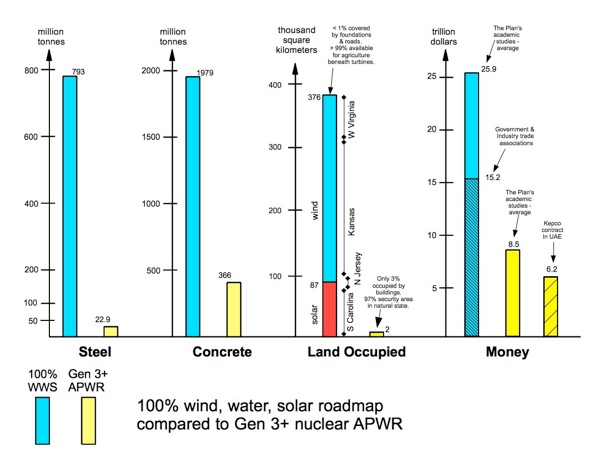
If we discover through the years that we must maintain our national overbuild ratio at its present 2.5 X value in order to ensure always-on status for everybody and everything in our entire primary energy economy, then all nuclear use-figures will rise by that same factor because we'll need to build

2.5 X 1376 = 3440 reactors.

At $6.2 B apiece, we would pay 3440 X $6.2 B = $21.3 trillion.  A huge amount to be sure, but better than the $60 trillion that we were staring at with my 4 X estimated overbuild of intermittent renewables.

Besides, aren't we hoping to install distributed SMRs in individual neighborhoods?  Power to the people, as it were.  No more long-distance sharing of dispatchable power among various geographic regions.

If that distributed local generation plan becomes our national model, we'll very likely be able to reduce our overbuild factor to less than its present 2.5 X. In that situation we can expect some savings on the $21.3 trillion expenditure in the paragraph above.

Keep in mind, Generation 3+ nuclear reactors by Westinghouse are not a futuristic technology like hydrogen-fueled transportation, for example. The first AP1000 reactor at Sanmen has finished construction and is now undergoing reduced-temperature testing of its piping systems. It's expected to begin generating power in 2017.69

Gen 3+ small modular reactors are technologically the same as full-scale AP1000s . There is no technical barrier to their integration into our energy system at a fraction of the cost of the 100% WWS Plan. And no problem finding room to put them.

What About Generation 4

Molten-Salt Reactors - MSRs?

Sure, let's get cracking on them. The scientific proof-of-concept has been demonstrated in the 1960s at Oak Ridge National Laboratory - ORNL.70

The fuel, thorium, is cheap and inexhaustible. It makes up 13 parts per billion of the entire Earth crust.

An MSR can't melt down because the fuel is already liquid. It can't suffer a steam- or hydrogen-explosion because it doesn't use any water, so there's no source of hydrogen.

Because it achieves 100% fissioning, "burn-up", of its fuel, an MSR doesn't produce any heavy-atom waste. That's quite unlike solid-fuel uranium reactors like the AP1000, which achieve only about 3% burn-up of their fissionable uranium. Their other 97% goes into spent-fuel storage. The only "waste" from an MSR is a small amount of non-fissionable radioactive medium-weight atoms, about 1 cubic foot volume per year of operation.71

MSRs are the ideal solution to the problem of what to do with unfissioned heavy atoms, uranium and plutonium, which are now sitting in cooling ponds inside spent fuel-rods. We can open those fuel-rods to extract the unfissioned uranium and plutonium, then feed those heavy atoms into an MSR, causing them to fission.  As in, they won't exist anymore.

Radiation leakage? If MSR fuel ever leaked, which it won't because it operates at only atmospheric pressure, the liquid would just lie on the floor in a puddle until it cooled and solidified. It's not a gas, so it can't drift away into the atmosphere.

This technology will be inexpensive to build because it doesn't have:

a) high-pressure plumbing;

b) backup cooling pumps to remove decay heat if the chain-reaction ever stops, since the liquid fuel would simply flow by gravity into a dump tank where it will cool at its own leisurely rate until it solidifies;

c) stainless-steel pressure vessel to contain a hydrogen explosion and drifting gases (Fukushima event), since there's no hydrogen anywhere nearby;

d) steam condenser to convert turbine exhaust steam into liquid water in preparation for reheating for its next pass through the turbine. MSR won't use steam for its turbine fluid. It will instead use a high-temperature gas like helium.

So MSR is safe, cheap, eliminates other peoples’ radioactive waste, and comes with enough thorium fuel on the planet to last forever. What's not to like?

Dear 100% WWS advocates: thanks for your good intentions and for your bold attempt to change not just electricity, but our entire PRI NRG supply away from fossils.  But let's skip the hassle of windmills and solar panels.  The Thorium Energy Alliance has got a better idea.

Footnotes

For convenience, footnotes can also be viewed separately on adjacent webpage.

1. http://thesolutionsproject.org/

2.  http://www.scientificamerican.com/article/a-path-to-sustainable-energy-by-2030/

https://web.stanford.edu/group/efmh/jacobson/Articles/I/sad1109Jaco5p.indd.pdf

3.  https://web.stanford.edu/group/efmh/jacobson/Articles/I/USStatesWWS.pdf

The Plan

4.  http://web.stanford.edu/group/efmh/jacobson/Articles/I/CombiningRenew/CONUSGridIntegration.pdf

http://tinyurl.com/z9e5dzm

Low-cost solution to the grid reliability problem with 100% penetration of intermittent wind, water, and solar for all purposes, pages 1, 2, 4

5. http://me1065.wikidot.com/ap1000

http://tinyurl.com/gktuzku

6. http://thorconpower.com/

http://flibe-energy.com/

http://www.transatomicpower.com/

http://terrapower.com/

7.  http://terrestrialenergy.com/

8.  http://energyfromthorium.com/2011/01/30/china-initiates-tmsr/

https://www.technologyreview.com/s/542526/china-details-next-gen-nuclear-reactor-program/

9.  http://search.usa.gov/search?utf8=%E2%9C%93&affiliate=eia.doe.gov&query=existcapacity_annual.xls

Then click or copy & paste first [XLS] www.eia.gov into browser; Open or Save the offered file; a spreadsheet doc will come up; scroll to line 38851 year 2015, All Sources, Nameplate Capacity 1,167,365  (1167 GW); Summer Capacity 1,064,054 megawatts  (1064 GW)

Alternatively, copy and paste into browser

US nameplate & summer electric capacity - all sources code H37306 line 37065.xls

Click Combined Heat and Power link; Open or Save the offered file; that same spreadsheet doc will come up; scroll to line 38851

All Sources total is followed by other energy sources used by Electric Power Industry: Coal, Geothermal, Hydro (conventional dammed), Natural Gas, Nuclear, combine Other Biomass with Wood and Wood-Derived Fuels, Petroleum, Pumped hydro energy storage - PHES, Solar Thermal and Photovoltaic are lumped together, Wind.

US wind capacity at end of 2015 was 73.4 GW; line 38863;

after 2015 addition of 8.6 GW. 

US utility-scale solar capacity, PV and CSP combined, at end of 2015 was 13.76 GWac; line 38862;

after 2015 addition of 6.2 GWac

10.  http://www.eia.gov/totalenergy/data/monthly/pdf/sec7_5.pdf

Table 7.2a, 2015, total = 4,087,381e6 kW-h; 4087.4e12 Wh ÷  8760 hr /yr = 466.6e9 W-y, 467 GW-y

11.  http://www.eia.gov/electricity/annual/html/epa_08_06_a.html

Table 8.6.A, 2012, contiguous US = 767,762 megawatts

12.  http://www.eia.gov/totalenergy/data/monthly/pdf/sec7_5.pdf

for 2015:

utility-scale solar actual NRG = 26,473 GW-h (PV and CSP); 

utility solar capacity (PV and CSP) = 13.76 GWp (footnote No. 9); 

utility solar NRG potential = 13.76 GW  X 8760 hr /yr = 120,500 GW-h; 

utility solar CF = 26,473 GW-h ÷ 120,500 GW-h = 21.9%

wind actual NRG = 190,927 GW-h;  

wind capacity = 73.4 GWp (footnote No. 9); 

wind NRG potential = 73.4 GW  X 8760 hr /yr = 643,000 GW-h; 

wind CF = 190,927 GW-h ÷ 643,000 GW-h = 29.7% 

12.3 www.seia.org/research-resources/solar-industry-data

p. 1; vertical axis scale factor is 61.1 MWac per mm;  ruler-scale all green-color bar heights from 2005–2015, then add those eleven measurements to obtain 90.5 mm; multiply 90.5 mm X 61.1 MW /mm = 5530 MW or 5.53 GW capacity, residential placement

12.4.  http://www.eia.gov/totalenergy/data/monthly/pdf/sec10_10.pdf

Table 10.6, row 2015 Total

Residential sector = 6999 GW-h;

12.5  Ibid. 12.3  www.seia.org/research-resources/solar-industry-data

p. 1; vertical axis scale factor is 61.1 MWac per mm;  ruler-scale all red-color bar heights from 2005–2015, then add those eleven measurements to obtain 98.2 mm; multiply 98.2 mm X 61.1 MW /mm = 6000 MW or 6.00 GW capacity, commercial placement

12.6  Ibid. 12.4   http://www.eia.gov/totalenergy/data/monthly/pdf/sec10_10.pdf

Table 10.6, row 2015 Total, columns 2 and 3

Commercial + Industrial sectors = 5689 + 1451 = 7140 GW-h

12.8  www.thesolutionsproject.org/resource/50-state-visions-infographics/

Download 50states_PDFs_all ; open the folder named 50states_PDFs_all; double-click the pdf icons for those 8 states; record from each state’s graphic the percentages of that state’s total Primary Energy to be provided by 1) Solar PV plants, and 2) CSP plants.

Add these percentages to obtain utility solar’s contribution to that state’s Primary Energy (all 4 sectors - electric, transport, heating /cooling, industry)

12.9  Find each state’s Primary Energy consumption in year 2013 by entering in browser bar

https://knoema.com/atlas/United-States-of-America/New-York/Energy-consumption

Record the large-font number at upper-left which is New York’s PRI NRG in units of billions of BTUs.  Move the decimal point 6 places to the left to express in units of quadrillion BTUs, called Quads, unit-symbol Q.

Multiply by the conversion factor 293 TWh /Q to convert to terawatt-hour units for Primary Energy.

Repeat this process 7 more times by replacing New-York with the other states’ names in the browser bar.  New-Jersey is hyphenated.

Multiply each state’s 2013 Primary Energy by the following factors to obtain its estimated Primary Energy demand in year 2050, per Table 1 of the Plan (footnote 3). 

NY = 0.636; NJ = 0.572; PA = 0.628; OH = 0.615; IN = 0.628; IL = 0.619; MI = 0.616; WI = 0.640.

Multiply each state’s estimated PRI NRG by the solar percentage obtained for it from the operation in footnote 12.8.  That gives each state’s utility-scale solar-supplied energy in 2050 in TWh units. 

Add all 8 states solar consumption to obtain 1709 TWh in year 2050.  Divide 1709 TWh by 5300 TWh to obtain 32.2%. 

The value 5300 TWh is obtained from the Plan’s Table 2 by adding column 2 in rows 9 and 10 to get 38.03%, then multiplying 38.03% X 13,937 TWh to get 5300 TWh.  The value 13,937 TWh is the Plan’s standard-demand load, 1591 GW-y, converted into TWh units by multiplying X 8760 hours /yr.

This calculation is valid only if the PV and CSP solar nameplate capacities in column 3 of rows 9 and 10 of Table 2 really do succeed in raising their capacity factor higher than 21.9%, which was their actual performance in 2015.

To the extent that they are unable to do so, those rows will be stuck providing utility-solar energy at their present CF level, which would be 2,553,300 MWp-ac X 8760 hr /y X 21.9% CF = 4070 TWh of electric energy in 2050 for the whole USA. 

To the extent the lower 21.9% capacity factor prevails, the percentage of utility solar that must be allocated to these northern 8 states must approach closer to 42%, not just 32%.  [1709 TWh (8 states in 2050) ÷ 4070 TWh (USA in 2050) = 0.420 or 42%]

13.    http://apps2.eere.energy.gov/wind/windexchange/wind_installed_capacity.asp     (interactive: click spreadsheet or annual maps) Installed Wind Capacity, US annual to 2015

14.  http://www.seia.org/research-resources/solar-industry-data 

third bar graph - US solar annual installed

http://www.seia.org/news/us-solar-market-sets-new-record-installing-73-gw-solar-pv-2015 

first bar graph   Note that the bar graph is expressed in dc watts.  Grid capacities are expressed in ac watts.  For conversion, assume ac-to-dc inverter conversion efficiency = 0.85 (85%).  7.286 GWdc X 0.85 = 6.19 GWac

Alternatively

http://tinyurl.com/jjhqsg6

smi-2015.pdf

15.  http://www.eia.gov/totalenergy/data/monthly/pdf/sec7_5.pdf     

190,927 GW-h ÷ 8760 hr /yr = 21.8 GW-y

16.  Ibid.      26,473 GW-h ÷ 8760 hr /yr = 3.0 GW-y

17.  Ibid.      251,168 GW-h = 28.7 GW-y

18.  Ibid.      1,335,068 GW-h = 152.4 GW-y

19.  http://www.eia.gov/dnav/ng/ng_cons_sum_dcu_nus_a.htm

20.  Ibid.   (residential + commercial + industrial values)

21.  http://apps2.eere.energy.gov/wind/windexchange/wind_installed_capacity.asp 

Ibid. No. 13

22.  http://www.nrel.gov/docs/fy13osti/56290.pdf  

p. v, Table ES-1, Summary of Land-Use Requirements for PV and CSP Projects in the United States

Direct Area,  Capacity-weighted average Land Use,  Large PV

22.3  https://www.choice.com.au/home-improvement/energy-saving/solar/review-and-compare/solar-panels

choose  Sunpower SPR-E20-327

navigate to    http://www.solardesigntool.com/components/module-panel-solar/Sunpower/2494/SPR-E20-327/specification-data-sheet.html

STC Power Rating: 327 Wdc

PTC Power Rating: 301.4 W; 

PTC derate factor = 0.922;   301.4 W ÷ 327 W  = 0.922

STC Power per unit of area:  200.5 W /m2

so derated PTC Power per unit of area = 0.922 X 200.5 = 185 Wdc /m2

dc-to-ac conversion at 0.85 efficiency;  0.85 X 185 Wdc /m2 = 157 Wac /m2

Round to 160 Wac /m2 for discussion & estimation

22.5  Panels' nominal power ratings, which are greater than 160 W /m2, are expressed for Standard Test Conditions and refer to dc electric output, which is incompatible with society’s mostly ac electric loads. Devices such as induction motors, lights, coiled heating elements, transformer-operated power supplies for battery-chargers and consumer electronic devices.

In other words, there are at least three possible quantifications for photovoltaic surface power density.  They are 1) STC-dc;  2) PTC-dc;  and 3) PTC-ac.  Only PTC-ac is useful for land area discussion.

In 2016 the best quality mass-production panel, when newly installed, has about 160 W /m2, rated PTC-ac.  Age degradation occurs at rates from 0.25% to 1% per year. At the end of an assumed 40-year lifetime such a panel will have declined to 96 –144 W /m2.

22.7  Ibid. No. 22

p. 12, Sec. 4.2.1, Evaluation of PV Packing Factors;

p. 13, Figure 7, Capacity-weighted average packing factor for PV projects

22.8  The area between rows (panel edge to panel edge) is somewhat greater than 60,000 m2 because of the plumb trigonometry of the panels’ tilt angle.

23.  For fixed mount:  http://c.ymcdn.com/sites/www.aec.org/resource/resmgr/PDFs/WhitePaper_IBISAECAluminumSo.pdf 

p. 6, Table 5, System Shipping Costs, Large Utility Ground Mount

Table 5 values are in English pounds, and refer to panel nominal (dc) kilowatts.  Divide material value by 0.85 , dc /ac conversion efficiency,  to relate to electric grid (ac) watts.   For fixed-mount, 73 tonnes steel /MWp-ac:

6,835,683 pounds ÷ 50,000 kW = 137 pounds /kWac; 137 ÷ 2.204 pounds /kg =62 kg /kWdc = 62 tonnes steel /MWdc; divide 62 tonnes by 0.85 for 73 tonnes steel /MWac

For tracking-mount:  https://us.sunpower.com/sites/sunpower/files/media-library/white-papers/wp-levelized-cost-drivers-electricity-utility-scale-photovoltaics.pdf  

p. 14, Figure 12  Area Related Cost Components for a T20 Tracker Power Plant

Figure 12 values are in English tons, and refer to panel nominal (dc) kilowatts.  Divide material values by 0.85 for ac.  For tracking-mount, 88 tonnes steel /MWp-ac:

35,083 tons ÷ 423,191 kWdc = 0.0828 ton /kWdc;  0.0828 ton ÷ 1.102 tons /tonne = 0.0751 tonne /kWdc = 75.1 tonnes steel /MWdc;  75.1 t ÷ 0.85 = 88 tonnes steel /MWac

23.2.  http://www.nrel.gov/docs/fy12osti/51664.pdf

p. 16-17

https://us.sunpower.com/sites/sunpower/files/media-library/data-sheets/ds-e20-series-327-residential-solar-panels-datasheet.pdf

23.5.  https://us.sunpower.com/sites/sunpower/files/media-library/white-papers/wp-sunpower-module-40-year-useful-life.pdf

24.  http://www.nrel.gov/docs/fy16osti/67142.pdf

p. 8, Overall Model Results, Utility Scale PV;  2016 fixed-tilt cost = $1.42 per dc watt.  Divide by 0.83 for ac.

$1.42 /Wdc ÷ 0.83 = $1.71 /Wac  (fixed-tilt in 2016)

{Our $1.71 /Wac contradicts the NREL study’s own Conclusion on p. 45, which states $1.99 /Wac for fixed-tilt utility farms.  NREL’s conclusion was based on the assumption that fixed-tilt farms, unlike tracking-mount farms, would use “oversized” central inverter equipment, presumably only one inverter station instead of several, to convert the farm’s output into ac power with very poor conversion efficiency of 71%.

This was an arbitrary assumption, it seems to the author, since NREL felt free to assume non-“oversized” central inverter technology for tracking-mount farms.  By doing so, achieving a more usual 83% conversion efficiency in the range that we have come to expect.

The author has reversed NREL’s “oversized” assumption for fixed-tilt farms’ inverter equipment.  Now expecting 83% dc-to-ac conversion for both mounting types.}

25.  Ibid.

p. 45, Conclusions (1);

$1.49 /Wdc ÷ 0.83 = $1.79 /Wac  (single-axis tracking in 2016)

26.  Ibid. 

$1.42 for fixed-tilt and $1.49 for tracking-mount, per dc watt.  Combined average $1.45 per dc watt.

p. 36, Utility Scale PV, Modeling Inputs;

Module Price:

$0.64 ÷ $1.42 = 45% for fixed mount

$0.64 ÷ $1.49 = 43% for tracking mount

44% average

Inverter Price:

$0.09 ÷ $1.42 = 6.3% for fixed mount

$0.10 ÷ $1.49 = 6.7% for tracking mount

6.5% average; round to 7%

Installation Labor:

http://www.nrel.gov/docs/fy15osti/64746.pdffor 2015 installations

See p.29, Figure 21

$0.16 /Wdc  for fixed mount

$0.22 /Wdc  for tracking mount

$0.19 /Wdc  average labor cost in 2015

Labor cost declined by about one-third from 2015 to 2016.  See NREL 2016 report. p. 8.  Compare orange-color segments in the bar graphs for those two years.  $0.19 declined to about $0.13 /Wdc.

$0.13 /Wdc ÷ $1.45 /Wdc = 9.0% for labor

27. Derivations of Table 2’s implied capacity factors for the three PV solar placements: utility-scale, residential roof, and commercial flat-roof:

Utility-Scale:  In row 9’s PV utility, 30.73% X 1591 GW all-purpose load gives 488.9 GWavg, or 488.9 GW-y /year in energy units.

With nameplate capacity of “2,326,000 MW”, the Plan’s PV farms have energy potential of 2326 GW-y /year if the sun shined all the time. 

Nameplate capacity values for utility-scale solar are almost always expressed in grid-compatible ac units.  This nameplate capacity value ought to be written more explicitly as “2,326,000 MWp-ac”.

Implied CF = 488.9 GW-y ÷ 2326 GW-y = 21.0% implied.

Combined PV and CSP actual utility-solar CF in 2015 was 21.9%, as derived in footnote 12. Thus the Plan’s presumption for utility PV production in row 9 is reasonable.  In fact, for mid- and long-term planning, if we could restrict utility solar farms to high insolation locations, especially our southwest, we could expect nationwide average PV solar capacity factor to rise into the mid-twenties.  For example, recent performances by three large PV farms in Southern California, namely Solar Star, Topaz, and Desert Sunlight, show capacity factors ranging from 24.5% to 26.7%. 

Residential: Nameplate capacities of residential rooftop solar are stated in dc power units, not ac units as for utility-scale projects. The value 379,500 MW in row 7 of Table 2 represents dc watt units.  The 100% WWS Plan specifies dc watts in Table 4 on p. 8, and also acknowledges dc units in the final paragraph of Section 5.2 on p. 10.

Using the standard 85% dc /ac conversion efficiency for less dusty rooftop placement, this represents 0.85 X 379,500 = 322,575 MWp-ac, or 322.6 GWp-ac.

If the sun shined 100% of the time, the row 7 national residential equipment would have potential annual energy of 322.6 GW-y /year. In order to achieve actual annual energy of 63 GW-y, residential solar would require CF = 63 GW-y ÷ 322.6 GW-y = 19.5% implied.

That is an unreasonable expectation (objection) for a nationwide residential average, in this author’s opinion.  It is probably impossible for nationwide residential solar CF to rise above its 2015 value of 14.4% derived in the Overview section.  This is because of south-siting issues, many sloped roofs having unfavorable angle of tilt, and partial shading by trees and other buildings, as mentioned there.

Commercial flat-roof:  Commercial rooftop solar, like residential, is specified in dc watt units, per Table 4 on p.8 of the 100% WWS Plan.

So row 8’s solar panel capacity of 276,500 MWp-dc converts to 0.85 X 276,500 MW =  235.0 GWp-ac, using 85% efficiency rule-of-thumb.

From column 4, “Percent of 2050 all-purpose load”, 3.24% X 1591 GW anticipates  51.5 GW-y /year. Implied capacity factor is given by CF = 51.5 GW-y ÷ 235.0 GW-y = 21.9%.

In high-insolation regions individual commercial rooftops can achieve capacity factors in the low- to mid-twenties range, comparable to ground-mount utility installations.  But it is not plausible as a nationwide average, with most commercial facilities concentrated in low-insolation regions.  2015’s commercial rooftop solar CF of only 13.6% resulted in a  shortfall of 19.5 GW-y, as derived in the Overview section. Therefore 51.5 GW-y annual energy production in row 8 is unreasonably optimistic.

28.  http://www.nrel.gov/docs/fy16osti/67142.pdf

p. 8, Overall Model Results; all values are expressed in dc watts,           

29.  Ibid.

p. 25, Residential PV: Modeling Inputs and Assumptions;

module + string inverter + installation labor =  $0.64 + $0.16 + $0.30 = $1.10.  22% + 6% + 10% = 38%

p. 8, bar graph; Scale orange segment for labor, 2.7 mm.  Vertical scale factor = $0.11 per mm. 

2.7 mm X $0.11 = $0.30 for labor

29.1. Ibid.

Inverter: 6%

Assume labor cost divides as 5% for panels and 5% for inverters. 

One inverter replacement: 6% + 5% = 11%.  Three additional replacements: 3 X 11% = 33%.

30.  http://c.ymcdn.com/sites/www.aec.org/resource/resmgr/PDFs/WhitePaper_IBISAECAluminumSo.pdf 

p. 6, Table 5,  System Shipping Costs

Table 5 values are in English pounds, and refer to panel nominal (dc) kilowatts, compatible with the Plan’s Table 2, row 8.

28,000 pounds steel ÷ 80 kW = 350 pounds /kWdc;  350 pounds ÷ 2.204 pound /kg =   159 kg steel /kWdc

31.  Ibid. No. 28

p. 8, Overall Model Results; commercial PV cost = $2.13 /Wdc

32.  Ibid.

p. 31, Commercial PV: Modeling Inputs and Assumptions;

module + inverter + installation labor = $0.64 + $0.13 + $0.20 = $0.97 /Wdc.  30% + 6% + 10% = 46%

p. 8, bar graph; Scale orange segment for labor.  1.8 mm X $0.11 /mm = $0.20

32.1.  Ibid. No. 29.5. 

Same inverter parts and labor percentages for commercial rooftop: 6% (parts) + 5% (labor) = 11%.

Three additional inverter replacements: 3 X 11% = 33%.

32.5   www.nrel.gov/docs/fy15osti/64898.pdf

p.5, Average US PV System Prices over Time;

Vertical axis scale factor = $0.20 per mm (20 cents per mm)

Apply ruler scaling to the final three green boxes; measure their centers below the $2 grid line and apply 20 cents /mm scale factor.

For residential and commercial combined, use the final 3 gray boxes for 2016, 2017 and 2018. Ruler-scale the center of each box relative to the $2 grid line.

32.7   Ibid. No. 24

p.42, Model Application-Module Efficiency Inputs; blue data points (bottom curve);

Vertical axis scale factor = $0.035 per mm (3.5 cents /mm)

At today's (CA) 16.7% solar conversion efficiency (5 mm to the right of 15% on horizontal axis), project up and over to vertical axis; the intercept scales to $1.42 /Wdc.

Repeat for 25% on horizontal axis; vertical intercept scales to $1.32 /Wdc; divide by $1.42 /Wdc = 0.930, a reduction of 7%.

Repeat the procedure for commercial (yellow curve), and for residential (brown).

33.  http://www.nrel.gov/docs/fy09osti/45834.pdf

p. 10, Table 1, Total Area, Average Area Requirements; expressed in hectare units (ha).  100 ha = 1 km2.  34.5 ha /MW = 0.345 km2 /MWp

34. http://www.windmatching.acroenergy.pl/turbine/227/

https://bravenewclimate.com/2009/10/18/tcase4/

Section 1.  Wind turbines;  daily material consumption based on 1160 wind turbines, model GE2.5xl.

335,000 t steel ÷ 1160 turbines = 289 t /turbine; 289 t /2.5 MW = 115.6 t steel /MWp

1,250,000 t concrete ÷ 1160 turbines = 1078 t /turbine; 1078 t /2.5 MW =                       431 t concrete /MWp

35. Technical Report NREL/TP-500-40566, http://www.nrel.gov/wind/pdfs/40566.pdf

Regarding blade mass: p. 11, Figure 1, graphs of blade mass versus blade length (called rotor radius) show exponents between 2.5 and 2.9, as do formulas appearing in figure caption below;

Regarding blade cost: p. 12, Figure 2, cost graphs and figure caption formulas show exponents from 2.5 up to 3 (cubed power);

Regarding tower and foundation mass: p. 20, Figure 3, graph of total mass is proportional (straight-line, or linear) with product of swept area X height.  Swept area and tower height tend to increase in tandem with design increases in turbine nameplate capacity  So the proportional graph indicates an approximate cubed function verse rotor radius (horizontal-axis units are cubic meters).

36. https://www3.epa.gov/climatechange/ghgemissions/usinventoryreport.html

U.S. Greenhouse Gas Inventory Report: 1990-2014; Overview of Greenhouse Gases and Sources of Emissions, first paragraph

http://tinyurl.com/h9jov6p

scroll to U.S. Greenhouse Gas Emissions by Economic Sector, 1990 - 2014

37.  http://newscenter.lbl.gov/2015/08/10/study-finds-that-the-price-of-wind-energy-in-the-united-states-is-at-an-all-time-low-averaging-under-2-5%C2%A2kwh/

Sixth paragraph, $1710 /kW

lbl.gov is Lawrence Berkeley Lab, affiliate of US DOE and Univ. of California

38.  Ibid.

Fifth paragraph

39.  https://www.irena.org/documentdownloads/publications/re_technologies_cost_analysis-wind_power.pdf

p. 35, seventh paragraph

40.  Correspondence thread with

Alfonso Alvaro

Corporate Director Strategy & Development

repoweringsolutions.com

A division of JERANEAS COMPANY

Refurbish wind turbine

The $4.7 M cost is for a slightly larger turbine than the 2-MW unit quoted.

41.  https://www.irena.org/documentdownloads/publications/re_technologies_cost_analysis-wind_power.pdf

p. 19, Table 4.1, Capital Investment Costs;  Onshore : Offshore ratio = 1 : 2

42.  http://www.aweo.org/windarea.html

From the list titled Areas of industrial wind facilities, the offshore wind farms have been extracted and are recorded here.  On-line, the projects are listed alphabetically by location, first in the US (Delaware and Massachusetts).  Then outside the USA (Br Col, Canada through UK) .

Winergy offshore, Del1,101 MW /67 mi2 

Cape Wind (off shore), Mass.420 MW /24 mi2 

Naikun Offshore, Hecate Strait, Br. Col.396 MW /100 km2

Horns Rev (off shore), Denmark160 MW /24 mi2 

Horns Rev II (off shore), Denmark209 MW /35 mi2

Butendiek (off shore), Germany240 MW /35 km2

Duddon Sands (off shore), U.K.500 MW /66 km2

London Array (off shore)1,000 MW /245 km2

Walney (off shore), U.K.450 MW /74.5 km2

Average4.36 MW /km2  = 0.229 km2 /MW

43. https://en.wikipedia.org/wiki/Andasol_Solar_Power_Station

https://www.rwe.com/web/cms/mediablob/en/1115150/data/0/1/Further-information-about-Andasol.pdf

p. 8, Data about the Andasol power plants (Data per power plant); forecast gross electricity volume: about 180 GWh (X 3) = 540 GWh /yr

http://www.power-technology.com/projects/andasolsolarpower/       second paragraph; “The three units have a net electricity output of 150 GWh per annum from each plant. The third plant was commissioned in September 2011. Andasol 3 is expected to produce   165 million kilowatt hours of electricity every year.”

The author of the article contradicts himself in these contiguous sentences.  The second sentence is the correct one; it is correct also regarding Andasol 1 and 2, since all three Andasol units are identical.  3 X 165 = 495 GWh /yr for entire Andasol.

44. https://www.rwe.com/web/cms/mediablob/en/1115150/data/0/1/Further-information-about-Andasol.pdf   

page 8,  Table labeled: Data about the Andasol power plants (Data per power plant); Terrain: approx 195 hectares (X 3) = 585 ha = 5.85 km2

45.  From    http://www.needs-project.org/docs/results/RS1a/RS1a%20D12.2%20Final%20report%20concentrating%20solar%20thermal%20power%20plants.pdf   page 88,

referenced in        https://bravenewclimate.com/2009/10/18/tcase4/

Section 2. Solar thermal.  fifth paragraph

690,000 t steel / 680 MWavg X 56.5 MWavg (Andasol) = 57,300 tonnes steel used by Andasol

2,215,000 t concrete / 680 MWavg X 56.5 MWavg (Andasol) = 184,000 tonnes concrete used by Andasol

46.  Ibid. No. 3, The 100% WWS Plan, Table S14, p. 91-92

Utility CSP w /storage:

Near-term values: 6148, 7535, 6000, 8500;  average $7046 /kW

Future values:  5016, 3500, 6000; average $4839 /kW

47.  http://www.power-technology.com/projects/andasolsolarpower/

first paragraph

https://en.wikipedia.org/wiki/Andasol_Solar_Power_Station  

Description section, third paragraph

48.  Ibid. No. 45

Utility PV fixed: Near-term and Future values:  1476, 2708, 1690, 3000, 1476, 2700, 1814, 1750; average $2077 /kWac

Utility PV tracking: Near-term and Future values:  3617, 1722, 2796, 3200, 3617, 1722, 2700, 3011, 2167, 1950, 3011;  average $2683 /kWac

Assuming 50 /50 split between fixed-mount and tracking-mount in future, combining fixed average $2077 with tracking average $2683 gives overall average for utility PV solar = $2380 /kWac

Residential PV: Near-term and Future values: 4427,6351, 3740, 4500, 3443, 3127, 2100; average $3955 /kWdc

Commercial PV: Near-term and Future values: 2951, 5113, 2390, 3500, 2459, 2796, 1900; average $3016 /kWdc

49.   The Plan’s authors explain the sources of the cost data that appear in Table S14 in a section titled ANNOTATION OF MAIN LITERATURE SOURCES USED IN OUR ANALYSIS OF THE NATIONAL-AVERAGE LCOE (TABLE S14), beginning on p. 107.  (LCOE - Levelized Cost of Energy)

In the EIA (Energy information Administration) subsection the authors state that near-term [cost] estimates are from Table 8.2 of EIA (2014a).  The Plan’s Table S14 near-term data entry is $3617 /kW, for tracking mount.  No entry is present in the Plan’s table for fixed mount.

However, EIA’s Table 8.2 Cost and Performance Characteristics of New Central Station Electricity Generating Technologies in 2014 shows $3394 /kW for base overnight cost and $3564 /kW for total overnight cost (with no distinction between fixed and tracking mount).  The Plan’s value $3617 /kW does not agree with EIA Table 8.2. 

EIA appends a footnote pertaining to its assumed 150-MW capacity (utility-scale) that “Costs and capacities are expressed in terms of net AC power available to the grid for the installed capacity.”   Meaning that costs are stated on an ac-watt basis, as is usual for utility-scale PV solar.

However, this ac-basis understanding is confounded in the subsection titled LBNL, Others on p. 109 [Lawrence Berkeley National Laboratory].  The Plan’s authors explicitly identify the data from the sources LBNL and others, at least, to state PV solar costs in per dc-watt units for all three placements, utility, commercial and residential;  second and third paragraphs.  This differs from the usual practice in non-academic publications, where utility-scale solar is described in ac-watt units.

So there is contradiction about the meaning of utility-scale PV solar costs in the Plan’s Table S14, as to whether the cost value refers to per dc-watt or per ac-watt units.  We will follow our former practice of interpreting utility-scale values on an ac-watt basis.  As usual, commercial and residential values are interpreted on a dc-watt basis.

50.  Ibid. No. 45 

From p. 92, Future wind

Onshore values:  1976, 1377, 2113;  average $1822 /kWac

Offshore values: 5077, 3050, 3191; average $3773 /kWac

51.  https://www.eia.gov/totalenergy/data/monthly/pdf/mer.pdf  

U.S. Energy Information Administration / Monthly Energy Review, May 2016 , page 17, Table 1.7, Primary Energy Consumption;  also p. 7, Table 1.3

52.  http://www.eia.gov/totalenergy/data/monthly/pdf/sec7_5.pdf

Table 7.2a, for 2010:

hydro plus geo combined = 260,203  + 15,219 =   275,422 GW-h

Primary Energy (footnote 48) =97.48 Quads X 293.1e3 GW-h /Q = 28.6e6 GW-h PRI NRG;

275,422 GW-h ÷  28.6e6 GW-h = 0.96%

53.   Ibid.

For 2015:  hydro plus geo combined =  251,168 + 16,767 = 267,935 GW-h

Primary Energy (Ibid. No. 48) = 97.527 Quads X 293.1e3 GW-h /Q = 28.6e6 GW-h PRI NRG (virtually no change from 2010)

267,935 GW-h ÷  28.6e6 GW-h = 0.94%

54.  Ibid.

hydro 2010: 260,203 GW-h; hydro 2015: 251,167 GW-h; 

hydro has declined 3.5% in past 5 years

55. From FN 12, utility solar (PV + CSP) capacity = 13.76 GW; actual energy = 26,473 GW-h

From FN 12.3, residential capacity = 5.53 GW

From FN 12.4, residential actual energy = 6999 GW-h

From FN 12.5, commercial capacity = 6.00 GW

From FN 12.6, commercial (plus industrial) actual energy = 7140 GW-h

Total capacity, all 3 placements = 13.76 + 5.53 + 6.00 = 25.29 GW; potential = 25.29 GW X 8760 h =

221.5e12 W-h

Total actual energy = 26,473 + 6999 + 7140 = 40,612 GW-h

Overall solar capacity factor = Total actual energy ÷ potential = 40,612e9 W-h ÷ 221.5e12 W-h = 0.183 or 18.3%

56. Ibid. No. 12

57.  http://energy.gov/sites/prod/files/2015/08/f25/2014-Wind-Technologies-Market-Report-8.7.pdf

page vii, Performance Trends section, first and second paragraphs

58.  http://www.publicpurpose.com/freeway1.htm 

section Cost of IHS on approximately p. 7;  $329 B in 1996 dollars

http://stats.areppim.com/calc/calc_usdlrxdeflator.php

$329 B in 1996 dollars X 1.431 inflation = $471 B in 2015 dollars

59.  http://web.stanford.edu/group/efmh/jacobson/Articles/I/CombiningRenew/CONUSGridIntegration.pdf  

page 1

Ibid.  No. 4

http://tinyurl.com/z9e5dzm  

60.  Ibid.  No. 9

scroll to line 37065, year 2014

Alternatively

US nameplate & summer electric capacity - all sources code H37306 line 37065.xls

61.  http://www.eia.gov/electricity/annual/html/epa_08_06_a.html

Most recent year 2012

62.  http://www.westinghousenuclear.com/New-Plants/Small-Modular-Reactor

scroll to Westinghouse SMR features at a glance

http://www.energy.gov/ne/nuclear-reactor-technologies/small-modular-nuclear-reactors

first paragraph

63.  https://bravenewclimate.com/2009/10/18/tcase4/

Section 3: Nuclear fission

Assumptions by Dr. Barry Brook about model AP1000:  average power = 1154 MW X 91.5% CF = 1056 MWavg;

Building thesis is 680 MWavg per day.  So 680 MWavg /day ÷ 1056 MWavg /reactor = 0.6439 reactor per day.

Steel use = 10,000 t /day.  10,000 t /day ÷ 0.6439 reactor /day = 15,500 t steel per reactor

Concrete use = 160,000 t /day.  160,000 t /day ÷ 0.6439 reactor /day =  248,000 t concrete per reactor

Footprint about 150 X 150 meters, Land area = 0.022 km2

AP1000-dimension footprint.pdf

http://me1065.wikidot.com/ap1000

see Comparison of Important Nuclear Island Buildings under fourth major section Simplification of Power Plant Design

http://tinyurl.com/gktuzku

scroll to any of several relevant drawings

64. http://instituteforenergyresearch.org/analysis/china-building-nuclear-plants-u-s-quietly-closes-them/

fourth paragraph

http://www.forbes.com/sites/jamesconca/2015/10/22/china-shows-how-to-build-nuclear-reactors-fast-and-cheap/#7e0baba4d0b3

twelfth paragraph

 

https://en.wikipedia.org/wiki/Changjiang_Nuclear_Power_Plant 

Sidebar features

65.  http://thebreakthrough.org/index.php/programs/energy-and-climate/historical-construction-costs-of-global-nuclear-power-reactors

Section 2, South Korea tells a very different story;  Scatter graph: Overnight construction cost in KRW currency = 2,000,000 KRW per kilowatt = $1740 /kW.  One S. Korea KRW (Korean Won) = $0.000 87;   so 2,000,000 KRW /kW above = $1740 / kW;

normalized to AP1000, 1120e6 W X $1740 /1e3 W = $1.9 billion /reactor

http://www.powerengineeringint.com/articles/2014/01/south-korea-s-first-post-fukushima-nuclear-plant-to-cost-7bn.html

fourth paragraph

Two 1400-MW plants = 2800 MW total;  $7 billion ÷ 2800 MW = $2.50 /W;  $2.50 /W X 1120e6 W (AP1000) = $2.8 billion / reactor, a higher cost than indicated by scatter graph above.

65.5.  http://www.world-nuclear.org/information-library/country-profiles/countries-t-z/united-arab-emirates.aspx

Section:  Nuclear power programme in the UAE, 9th paragraph, $20.4 billion cost

$25 billion cost:

https://www.bloomberg.com/news/articles/2015-09-03/abu-dhabi-said-to-revive-debt-plan-for-first-nuclear-power-plant-ie3wyuib

https://en.wikipedia.org/wiki/APR-1400

Design section: Net electric power = 1400 MWe

66.  Ibid. No. 3, 100% WWS Plan,  https://web.stanford.edu/group/efmh/jacobson/Articles/I/USStatesWWS.pdf

16. p.91-92, Table S14;  Nuclear, Advanced Pressurized Water Reactor - APWR: Near term and Future values:  5583, 6640, 6511, 4434, 4279, 6511, 3800, 6500; average $5532 /kW
    

67. https://aris.iaea.org/sites/..%5CPDF%5CAP1000.pdf

p. 4, Section 2.2,  Reactor core and fuel design, third paragraph

http://www.westinghousenuclear.com/New-Plants/AP1000-PWR/Operations-and-Maintenance

first section: Improved Plant Performance

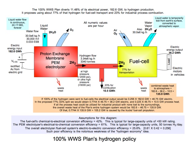
2016, June 22

Material Limits   

Steel and concrete are the main construction materials required for the WWS buildout, but they are not limiting factors.  There is enough of those two materials to complete the job.  Not necessarily so for certain other materials.

We will set aside the issue of lanthanides, so-called rare earth metals.  Their supply chains may occasionally become problematic because of their concentration in China and Brazil.  But with the comparatively small quantities of them required for solar and wind equipment, existing world reserves are sufficient to carry humankind forward even if all countries were to adopt the 100% WWS idea.

Copper is another matter because we need so much of it.  But the real problem is silver.

Material limits must be discussed only in the context of the entire world, not just the US.  In principle, to deal with climate disruption the WWS Plan must be embraced by all mankind. In that spirit the Solutions Project does propose an individualized plan for every large country.

The overall global WWS Plan is presented at http://thesolutionsproject.org/resource/transition-chart-to-100-clean-renewable-energy/ .  Download the first file, “Solutions-World-2015-Web”.  It is helpful to print that S-curve graph.

Find the Solutions Project’s global total solar power and total wind power by referring to the values on the right-side vertical axis.  Global average power is expected to be 11,797 GW.  That is an average value, not a peak capacity. 

As shown on the axis, solar is expected to provide 61.3% of the total, or 7230 GWavg.  PV and CSP are combined.

Wind, onshore and offshore, is expected to provide 32.3% of 11,797 GW, or 3810 GWavg. 

The Plan’s implied capacity factor for all PV solar in the US is about 21%.27  Extrapolating that CF to the entire world, global solar nameplate capacity must be 7230 GWavg ÷ 0.21 CF = 34,400 GWp-ac.

The Plan’s implied capacity factor for US onshore wind is 29%.  For offshore it’s 39%.50.2  With more onshore than offshore, their weighted average CF is 33%.  Extrapolating that CF to the entire world, global wind capacity must be  3810 GWavg ÷ 0.33 CF = 11,500 GWp, nameplate rating. 

The industry-standard values for copper usage are:50.3

Solar PV: 5 tonnes Cu per megawatt of peak capacity.  5 tonnes /MWp

Wind:  3 t /MWp

These can be restated to be consistent with our preferred GW units as:

Solar PV: 5,000 tonnes Cu per gigawatt of peak capacity.  5,000 tonnes /GWp

Wind:  3,000 t /GWp

We subsume CSP construction into PV construction globally, justified by extrapolating the 84% /16% split between PV and CSP in the US Plan.

Therefore the copper required globally through 2050 solar construction would be 34,400 GWp X 5,000 t Cu /GWp = 172,000,000  tonnes Cu. 

Required for global wind construction would be 11,500 GWp X 3,000 t Cu /GWp = 34,500,000 tonnes Cu. 

Total = 172,000,000 + 34,500,000 = 206,500,000 tonnes of copper through year 2050, for solar & wind construction globally.

Worldwide proved reserves of copper are 720,000,000 tonnes. Go to https://minerals.usgs.gov/minerals/pubs/commodity/copper/mcs-2017-coppe.pdf

On Frame 2, page 55, refer to the table World Mine Production and Reserves.  The units are thousands of tonnes.  In Reserves column, World total = 720,000,000 t.

Therefore the global WWS build-out would consume 29% of the world’s proved copper reserves. [206,500,000 t ÷ 720,000,000 t = 29%]

Whether the various on-going industrial and electrical uses of copper could continue functioning under such an immense diversion from copper-mine output cannot now be known.

Silver

Mined silver supplies have not yet been stressed by solar equipment demand because humans have built so little solar to date.  Worldwide, PV capacity was 303 GWp-ac at year-end 2016, and CSP was 4.8 GW, for a combined 308 GW.50.4  This is less than 1% of the Solutions Project’s 2050 goal of 34,400 GW, stated earlier.

Silver is an ingredient in the metal paste that forms the conducting fingers and busbars on the front surface of a photovoltaic cell. The silver content of crystalline silicon PV cells was about 31 milligrams per dc watt in 2016.50.5 This is a reduction from about 82 mg /Wdc in 2013, as solar manufacturers strive to minimize their silver consumption. 

The photovoltaic industry projects a steady reduction going forward.  It anticipates a goal of 13 mg /Wdc in 2026, the year when the world reaches the halfway point in total solar installation, per the Roadmap’s construction schedule.50.6  Therefore we can take 13 mg /W as the average silver usage rate for PV equipment over the 35-year plan duration, even if further reductions are achieved after 2026.

Extrapolating the US Roadmap’s 84% /16% split between PV and CSP,  total global solar of 34,400 GWp-ac breaks down into 28,900 GWp-ac for PV and 5,500 GW for CSP.

The photovoltaic cells themselves must have dc power capacity greater than 28,900 GW,  to allow for 85% conversion efficiency of the electronic inverters that convert dc to grid-compatible ac.  The global Roadmap’s PV infrastructure must have dc capacity given by 28,900 ÷ 0.85 = 34,000 GWdc.

Therefore silver consumption for all global PV solar cells through 2050 can be estimated as 34,000 GWdc X 13 mg /Wdc = 442,000 tonnes.

CSP solar collector mirrors use silver for their reflective coating, applied 100-nanometers thick on steel parabolic bases.  That requires 13 tonnes of silver per gigawatt of capacity.50.7  So for CSP, 5,500 GW X 13 t /GW = 72,000 additional tonnes of silver.  Combined PV and CSP = 442,000 t + 72,000 t = 514,000 t. 

The world’s proven silver reserves are 570,000 tonnes.50.8  The global Roadmap Plan would consume 90% of it.

Present non-solar industrial demand for silver is 15,700 tonnes annually.50.9  Even presuming no increase in global industrial demand despite the rapid industrialization of China, India and others, industrial consumption during the 35-year WWS buildout would be 35 yr X 15,700 t /yr = 550,000 t.

But only 56,000 tonnes of silver would remain in the ground after satisfying solar equipment usage of 514,000 t.

There isn’t enough silver on the planet to support the Solutions Project’s solar construction along with current industrial consumption.

Footnotes

50.2   https://web.stanford.edu/group/efmh/jacobson/Articles/I/USStatesWWS.pdf

The Solutions Project Roadmap Plan.  See Frame 8, page 6, Table 2. 

Onshore wind, row 1, column 3;  30.92% X 1591 GWavg = 492 GWavg.  Column 4, Name-plate capacity = 1,701,000 MWp.  CF = 492e9 Wavg ÷ 1,701,000e6 Wp = 0.289, or 29% onshore CF.

Offshore wind, row 2, column 3;  19.08% X 1591 GWavg = 304 GWavg.  Column 4, Name-plate capacity = 780,900 MWp.  CF = 304e9 Wavg ÷ 780,900e6 Wp = 0.389, or 39% offshore CF.

50.3

https://en.wikipedia.org/wiki/Copper_in_renewable_energy

Refer to the table “Copper usage in renewal energy generation”.  Power values are expressed in terms of peak capacity.

Photovoltaics row, columns 2 and 4. 

350 kilotonnes Cu ÷ 70 GWp cumulative installed PV solar = 350e3 tonnes ÷ 70e3 MWp = 5 tonnes Cu /MWp

Wind row, columns 2 and 4. 

714 kilotonnes Cu ÷ 238 GWp cumulative installed wind =  3 tonnes Cu /MWp

50.4

http://www.iea-pvps.org/fileadmin/dam/public/report/statistics/IEA-PVPS_-_A_Snapshot_of_Global_PV_-_1992-2016__1_.pdf

See page 7.

https://en.wikipedia.org/wiki/Concentrated_solar_power#Deployment_around_the_world

See table Worldwide Concentrated Solar Power.   4.815 GWp in 2016.

50.5

http://www.itrpv.net/Reports/Downloads/2016/

Refer to Fig. 8 on page 11, Frame 13.  The data point for 2016 indicates 95 milligrams of silver per cell (crystalline silicon technology).  Assuming power rating of 3.1 watts per cell, the usage of silver is 95 mg ÷  3.1 W = 31 mg /W. 

The reference PV unit is SunPower Co. module E20-435, containing 128 cells.  Module power rating = 401 Wdc under PTC (Photovoltaics for Utility-Scale Test Conditions, often referred to as Practical Test Conditions).  401 W ÷ 128 cells = 3.1 Wdc /cell.

It’s 435 W nominal rating refers to STC - Standard Test Conditions (laboratory). 

http://www.iom3.org/sites/default/files/iom3-corp/Mason%20SMEET%202%20presentation%2027Feb13.pdf

See page 11, referring to February 2013.  Silver price = $1.10 /gram.  Silver cost per PV watt (PTC) = $0.09.   

$0.09 /W ÷  $1.10 /g  = 0.082 g /W or 82 mg /W.

50.6

Ibid. Footnote 50.5. 

The data point for 2026 indicates 40 milligrams of silver per PV cell.  40 mg /cell ÷ 3.1 W /cell = 13 mg /W.

50.7

http://fossilhub.org/wp-content/uploads/2014/03/Pihl_etal2012_ConcSolarPower_materials.pdf

Material constraints for concentrating solar thermal power

See table 3 on page 5.  13 tonnes silver per GWac = 13e6 g /1e9 W = 13e–3 g /W = 13 mg /Wac

50.8

https://minerals.usgs.gov/minerals/pubs/commodity/silver/mcs-2017-silve.pdf

Refer to the first page. Units are tonnes.  Reserves column, world total = 570,000 tonnes of silver

50.9

http://www.silverinstitute.org/wp-content/uploads/2017/08/SilverInterim2016.pdf

See page 5, row Industrial Fabrication, column year 2016.  Units are millions of troy ounces (Moz).  The conversion factor is 31.1 tonnes per Moz.

585 Moz X 31.1 t /Moz = 18,200 t /yr.

https://www.bullionvault.com/gold-news/silver-solar-011120173

See the first bar graph, year 2016.  PV’s share is 14% X 18,200 t = 2,540 t.

18,200 t – 2,500 t = 15,700 t /yr.